R Programming Tutorial for Beginners

R Programming Tutorial for Beginners

R is a programming language and suite of tools for reporting, statistical analysis, and graphic depiction. This tutorial is intended for beginners and experienced programmers, statisticians, and data miners who want to learn how to create statistical software using R programming. 

Introduction to R Programming

• R is free software provided under a copy-left license in the GNU style.
• At the University of Auckland, New Zealand, Ross Ihaka and Robert Gentleman wrote the first version of R in the Department of Statistics. The first time R appeared was in 1993.

Features of R Programming

• R is an interpreted language.
• It offers efficient facilities for handling and storing data.
• It is a strong, highly expandable, open-source program.
• It offers graphical approaches that are very extensible.
• It enables us to use vectors to carry out several calculations. 
• Its collection of data analysis tools is integrated and consistent. 
• R includes a collection of operators for performing various arrays, lists, and vector calculations. 
• It is a well-developed programming language that is straightforward and efficient.
• It’s software for analyzing data.
• Its user-defined, looping, conditional, and diverse I/O facilities make it a well-designed, simple, and efficient language.

Real-time Applications of R Programming

Numerous real-time applications are accessible. Here are some of the well-liked applications:

• Facebook
• Google
• Twitter
• XBOX ONE
• Sunlight Foundation
• RealClimate
• NDAA
• FDA

The learning of R programming requires an understanding of any other programming language like C++, Java, Python, various graph types for data representation, and the knowledge of statistical theory in mathematics.

R Programming Installation

You can use the instructions below to build up your environment for R.

Windows Installation

R-3.2.2 for Windows (32/64 bit) is the Windows installer version that you can download and store in a local directory.

• “R-version-win.exe” is the name of the Windows installer (.exe). 
• Simply double-click the installer to launch it with the default settings applied. 
• It installs the 32-bit version of Windows.
• However, it installs both the 32-bit and 64-bit versions if your Windows version is 64-bit.
• The program icon can be found in Windows Program Files in the directory structure “R\R3.2.2\bin\i386\Rgui.exe” after installation. 
• The R-GUI, or R console, is displayed when you click this icon to begin R programming.

Linux Installation

R can be found at R Binaries, where it is provided as a binary for several Linux versions. 

• Installation instructions for Linux differ depending on the flavor. 
• If you’re pressed for time, you can install R using the yum command as follows:
  • $ yum install R
• The above command will install the essential R programming capability along with standard packages. 
• If you still require additional packages, you can launch the R prompt by doing the following:

$ R

R version 3.2.0 (2015-04-16) — “Full of  Ingredients”          

Copyright (C) 2015, The R Foundation for Statistical Computing

Platform: x86_64-redhat-linux-gnu (64-bit)

R is free software and comes with ABSOLUTELY NO WARRANTY.

You are welcome to redistribute it under certain conditions.

Type ‘license()’ or ‘licence()’ for distribution details.

R is a collaborative project with many contributors.                    

Type ‘contributors()’ for more information and

‘citation()’ on how to cite R or R packages in publications.

Type ‘demo()’ for some demos, ‘help()’ for on-line help, or

‘help.start()’ for an HTML browser interface to help.

Type ‘q()’ to quit R.

>  

• Installing the necessary package can now be done at the R line by using the install command. 
• For example, installing the plotrix package, which is necessary for 3D charts, can be done with the following command.
  • > install.packages(“plotrix”)

Basics of R Programming

You can write your program at the R command prompt or with an R script file, depending on your needs. Let’s explore each one separately.

R Command Prompt

After setting up your R environment, all you need to do is type the following command to launch your R command prompt:

$ R

After the R interpreter has been launched, you will see a prompt > where you may begin typing your program, as seen below:

> myString <- “Hello, World!”

> print ( myString)

[1] “Hello, World!”

The string variable myString is defined in the first sentence, to which the string “Hello, World!” is assigned. The value of the variable myString is then printed using the print() function in the next statement.

R Script File

The typical method of programming is to write your code in script files, which you can then run at the command prompt using the Rscript interpreter. 

Let us begin by putting the following code into a text file named test.

# My first program in R Programming

myString <- “Hello, World!”

print ( myString)

Put the code listed above in a test file. R and run it as instructed below at the Linux command prompt. The syntax won’t change whether you’re using Windows or another operating system.

$ Rscript test.R

The program mentioned above yields the following output when we run it.

[1] “Hello, World!”

Comments

When your program is running, the interpreter ignores comments; they work much like help text in an R application. The statement’s first comment is written with a # symbol, as follows:

# My first program in R Programming

R does not support multi-line comments; however, you can still accomplish the following trick:

if(FALSE) {

   “This is a demo for multi-line comments and it should be put inside either a 

      single OR double quote”

}

myString <- “Hello, World!”

print ( myString)

Output

[1] “Hello, World!”

The above remarks won’t affect your actual program, even though the R interpreter will execute them. Such remarks ought to be included, either as a single quote or as two quotes.

R Data Types

When variables are assigned using R-objects, the R-object’s data type is used as the variable’s data type. R-objects come in a variety of varieties. The most commonly utilized ones are:

• Vectors
• Lists
• Matrices
• Arrays
• Factors
• Data Frames

Vectors

The c() function, which combines the items into a vector, should be used to build vectors with many elements.

# Create a vector.

apple <- c(‘red’,’green’,”yellow”)

print(apple)

# Get the class of the vector.

print(class(apple))

Output:

[1] “red”    “green”  “yellow”

[1] “character”

Lists

A list is an R-object that can have vectors, functions, and even another list inside of it, among many other kinds of elements.

# Create a list.

list1 <- list(c(2,5,3),21.3,sin)

# Print the list.

print(list1)

Output

[[1]]

[1] 2 5 3

[[2]]

[1] 21.3

[[3]]

function (x)  .Primitive(“sin”)

Matrices

A rectangular, two-dimensional data set is called a matrix. A vector can be sent into the matrix function to create it. 

# Create a matrix.

M = matrix( c(‘a’,’a’,’b’,’c’,’b’,’a’), nrow = 2, ncol = 3, byrow = TRUE)

print(M)

Output

[,1] [,2] [,3]

[1,] “a”  “a”  “b” 

[2,] “c”  “b”  “a”

Arrays

The necessary number of dimensions is created via the array function, which accepts a dim property. The example below shows how to create an array with two 3×3 matrices as its members.

# Create an array.

a <- array(c(‘green’,’yellow’),dim = c(3,3,2))

print(a)

Output

, , 1

     [,1]     [,2]     [,3]    

[1,] “green”  “yellow” “green” 

[2,] “yellow” “green”  “yellow”

[3,] “green”  “yellow” “green” 

, , 2

     [,1]     [,2]     [,3]    

[1,] “yellow” “green”  “yellow”

[2,] “green”  “yellow” “green” 

[3,] “yellow” “green”  “yellow”  

Factors

A vector is used to produce the r-objects known as factors. The vector is stored together with the unique values that correspond to each member of the vector as labels. 

Factor() is the function used to produce factors. The level count is provided via the ‘nlevels’ function.

# Create a vector.

apple_colors <- c(‘green’,’green’,’yellow’,’red’,’red’,’red’,’green’)

# Create a factor object.

factor_apple <- factor(apple_colors)

# Print the factor.

print(factor_apple)

print(nlevels(factor_apple))

Output

[1] green  green  yellow red    red    red    green 

Levels: green red yellow

[1] 3

Data Frames

Tabular data items are called data frames. It is an equal-length vector list. The data.frame() function is used to build data frames.

# Create the data frame.

BMI <- data.frame(

   gender = c(“Male”, “Male”,”Female”), 

   height = c(152, 171.5, 165), 

   weight = c(81,93, 78),

   Age = c(42,38,26)

)

print(BMI)

Output

  gender height weight Age

1   Male  152.0     81  42

2   Male  171.5     93  38

3 Female  165.0     78  26  

R Variables

We can manipulate named storage with our applications due to variables. In R, a variable can hold one atomic vector, a collection of atomic vectors, or an amalgam of several Robjects.

Variable Assignment

The operators equal to, leftward, and rightward can be used to assign values to the variables. The print() or cat() functions can be used to print the values of the variables.

# Assignment using equal operator.

var.1 = c(0,1,2,3)           

# Assignment using leftward operator.

var.2 <- c(“learn”,”R”)   

# Assignment using rightward operator.   

c(TRUE,1) -> var.3           

print(var.1)

cat (“var.1 is “, var.1 ,”\n”)

cat (“var.2 is “, var.2 ,”\n”)

cat (“var.3 is “, var.3 ,”\n”)

Output

[1] 0 1 2 3

var.1 is  0 1 2 3 

var.2 is  learn R 

var.3 is  1 1 

Data Types of a Variable

R is a dynamically typed language, meaning that when utilizing a variable in a program, we can repeatedly alter its data type.

var_x <- “Hello”

cat(“The class of var_x is “,class(var_x),”\n”)

var_x <- 34.5

cat(”  Now the class of var_x is “,class(var_x),”\n”)

var_x <- 27L

cat(”   Next the class of var_x becomes “,class(var_x),”\n”)

Output

The class of var_x is  character 

   Now the class of var_x is  numeric 

      Next the class of var_x becomes  integer

Finding Variables

We utilize the ls() function to get the list of all the variables that are now available in the workspace. The ls() function can also match variable names using patterns.

print(ls())

Output

[1] “my var”     “my_new_var” “my_var”     “var.1”      

[5] “var.2”      “var.3”      “var.name”   “var_name2.”

[9] “var_x”      “varname” 

Deleting Variables

The rm() function can be used to remove variables. We removed the variable var.3 below. An error is raised when the variable’s value is printed.

rm(var.3)

print(var.3)

Output

[1] “var.3”

Error in print(var.3) : object ‘var.3’ not found

Using rm() and ls() combined will remove all of the variables.

rm(list = ls())

print(ls())

Output

character(0)

R Operators

An operator is a symbol that instructs the compiler to carry out particular logical or mathematical operations. The R programming language offers the following kinds of operators and has many built-in operators.

Types of Operators

In R programming, we have the following kinds of operators −

• Arithmetic Operators
• Relational Operators
• Logical Operators
• Assignment Operators
• Miscellaneous Operators

Arithmetic Operators

The arithmetic operators that the R language supports are displayed in the following table. 

+: Addition of Vectors

v <- c( 2,5.5,6)

t <- c(8, 3, 4)

print(v+t)

Output

[1] 10.0  8.5  10.0

-: Subtracts Vectors

v <- c( 2,5.5,6)

t <- c(8, 3, 4)

print(v-t)

Output

[1] -6.0  2.5  2.0

*: Multiplication

v <- c( 2,5.5,6)

t <- c(8, 3, 4)

print(v*t)

Output

[1] 16.0 16.5 24.0

/: Division

v <- c( 2,5.5,6)

t <- c(8, 3, 4)

print(v/t)

Output

[1] 0.250000 1.833333 1.500000

%%: Produce Reminders

v <- c( 2,5.5,6)

t <- c(8, 3, 4)

print(v%%t)

Output

[1] 2.0 2.5 2.0

%/%: Produce Quotient of Second Vector 

v <- c( 2,5.5,6)

t <- c(8, 3, 4)

print(v%/%t)

Output

[1] 0 1 1

^: Produce the exponent of the second vector.

v <- c( 2,5.5,6)

t <- c(8, 3, 4)

print(v^t)

Output

[1]  256.000  166.375 1296.000

Relational Operators

Every element in the first vector and its matching element in the second vector are compared. The relational operators that the R language supports are displayed below:

>: Greater Than

v <- c(2,5.5,6,9)

t <- c(8,2.5,14,9)

print(v>t)

Output

[1] FALSE  TRUE FALSE FALSE

<: Less Than

v <- c(2,5.5,6,9)

t <- c(8,2.5,14,9)

print(v < t)

Output

[1]  TRUE FALSE  TRUE FALSE

==: Equal To

v <- c(2,5.5,6,9)

t <- c(8,2.5,14,9)

print(v == t)

Output

[1] FALSE FALSE FALSE  TRUE

<=: Less than or equal to

v <- c(2,5.5,6,9)

t <- c(8,2.5,14,9)

print(v<=t)

Output

[1]  TRUE FALSE  TRUE  TRUE

>=: Greater than or equal to

v <- c(2,5.5,6,9)

t <- c(8,2.5,14,9)

print(v>=t)

Output

[1] FALSE  TRUE FALSE  TRUE

!=: Unequal

v <- c(2,5.5,6,9)

t <- c(8,2.5,14,9)

print(v!=t)

Output

[1]  TRUE  TRUE  TRUE FALSE

Logical Operators

Every element in the first vector and its matching element in the second vector are compared. A boolean value is the outcome of the comparison.

&: Element-wise Logical AND operator

v <- c(3,1,TRUE,2+3i)

t <- c(4,1,FALSE,2+3i)

print(v&t)

Output

[1]  TRUE  TRUE FALSE  TRUE

|: Element-wise Logical OR operator

v <- c(3,0,TRUE,2+2i)

t <- c(4,0,FALSE,2+3i)

print(v|t)

Output

[1]  TRUE FALSE  TRUE  TRUE

!: Logical NOT operator

v <- c(3,0,TRUE,2+2i)

print(!v)

Output

[1] FALSE  TRUE FALSE FALSE

&&: Logical AND

v <- c(3,0,TRUE,2+2i)

t <- c(1,3,TRUE,2+3i)

print(v&&t)

Output

[1] TRUE

||: Logical Operator

v <- c(0,0,TRUE,2+2i)

t <- c(0,3,TRUE,2+3i)

print(v||t)

Output

[1] FALSE

Assignment Operator

Vectors can be given values through the use of these operators.

<− or = or <<−: Left Assignment

v1 <- c(3,1,TRUE,2+3i)

v2 <<- c(3,1,TRUE,2+3i)

v3 = c(3,1,TRUE,2+3i)

print(v1)

print(v2)

print(v3)

Output

[1] 3+0i 1+0i 1+0i 2+3i

[1] 3+0i 1+0i 1+0i 2+3i

[1] 3+0i 1+0i 1+0i 2+3i

-> or ->>: Right Assignment

c(3,1,TRUE,2+3i) -> v1

c(3,1,TRUE,2+3i) ->> v2 

print(v1)

print(v2)

Output

[1] 3+0i 1+0i 1+0i 2+3i

[1] 3+0i 1+0i 1+0i 2+3i

Miscellaneous Operators

These operators are not used for broad mathematical or logical computations; rather, they are utilized for specific purposes.

:- Colon Operator

v <- 2:8

print(v) 

Output

[1] 2 3 4 5 6 7 8

%in%: Identification

v1 <- 8

v2 <- 12

t <- 1:10

print(v1 %in% t) 

print(v2 %in% t) 

Output

[1] TRUE [1] FALSE

%*%: Multiply Matrix

M = matrix( c(2,6,5,1,10,4), nrow = 2,ncol = 3,byrow = TRUE)

t = M %*% t(M)

print(t)

Output

      [,1] [,2]

[1,]   65   82

[2,]   82  117

Decision-Making in R Programming

Programmers who create decision-making structures must specify one or more conditions that the program will evaluate or test. 

A statement or statements that will be performed if the condition is found to be true, and optionally, additional statements that will be performed if the condition is found to be false.

if statement: An if statement is made up of one or more assertions and a Boolean expression.

Syntax

if(boolean_expression) {  

// Statement(s) will be carried out if the boolean expression is true.

}  

if…else statement: An optional else statement, which runs if the Boolean expression is false, can come after an if statement.

Syntax

if(boolean_expression 1) {  

   // This block executes when the boolean expression 1 is true.  

} else if( boolean_expression 2) {  

   // This block executes when the boolean expression 2 is true.  

} else if( boolean_expression 3) {  

   // This block executes when the boolean expression 3 is true.  

} else {  

   // This block executes when none of the above conditions is true.   

} 

switch statement: It is possible to compare a variable’s value to a list of values using a switch statement.

switch(expression, case1, case2, case3….)  

Control Statements in R Programming

For Loop: A vector can be iterated using a for loop. Here, the body is executed and the given condition is verified.

for (initialization_Statement; test_Expression; update_Statement)  

{  

    // statements inside the body of the loop   

}  

While Loop: One kind of control flow statement that is used to repeatedly cycle a piece of code is the while loop. The body of the statement will execute in a while loop after the condition has been checked.

while (test_expression) {  

   statement  

}  

Functions in R Programming

A function is a collection of statements arranged to carry out a certain function. In addition to offering many built-in functions, R lets users write custom functions.

func_name <- function(arg_1, arg_2, …) {  

   Function body   

}  

Components of Function

The function in R consists of the following four elements: 

• Function Name
• Arguments
• Function Body
• Return Value

Types of Function

R contains two different kinds of functions: built-in functions and user-defined functions, just like the other languages.

Built-in Functions in R

Built-in functions are those that are pre-defined or pre-created within the programming framework.

Numerous built-in functions in R, like sum(x), max(), mean(), and seq(), are available. 

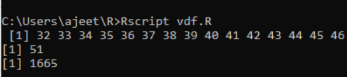
#Generating a 32–46 number sequence. 

print(seq(32,46))

# Calculating the average of the numbers between 22 and 80. 

print(mean(22:80))

# Calculating the total number between 41 and 70. 

print(sum(41:70))   

Output

User-defined Functions in R

We can write customized functions in our programs using R. We can utilize these functions like built-in functions after they are constructed.

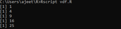
# Creating a function without an argument.  

new.function <- function() {  

   for(i in 1:5) {  

      print(i^2)  

   }  

}       

new.function()  

Output

Conclusion

We have covered all the basic concepts of the R programming language in this R programming tutorial. If you want to learn them from scratch with satisfying hands-on exposure, enroll in our R programming training in Chennai.